Plotting functions for geometries — euclid

euclid provide interfaces for both base and grid graphics that allows you to visualise the geometries you are working with. There is only functionality for 2D geometries so 3D geometries will be mapped to the plane given by the mapping_plane argument. The plot method for geometries will behave like the base plot() method and set up a new plotting window based on the given settings. euclid_plot will add to the existing plot and thus use the coordinate system currently in effect. euclid_grob will create a grob that can be rendered with grid.draw().

Usage

euclid_plot(x, ..., mapping_plane = "z")

euclid_grob(
  x,
  ...,
  unit = "native",
  name = NULL,
  gp = gpar(),
  vp = NULL,
  mapping_plane = "z"
)

# S3 method for euclid_geometry
plot(
  x,
  y,
  xlim = NULL,
  ylim = NULL,
  mapping_plane = "z",
  add = FALSE,
  axes = TRUE,
  frame.plot = axes,
  ...
)

Arguments

x

A geometry vector

...

Arguments passed along to the specific drawing method.

points (and weighted points) use points() and pointsGrob()
circles use symbols() and circleGrob()
directions and vectors use arrows() and segmentsGrob()
iso rectangles and bounding boxes use symbols() and rectGrob()
lines, rays, and segments use segments() and segmentsGrob()
triangles use polygon() and polygonGrob()

mapping_plane

either "x", "y", "z", or a scalar plane geometry

unit

The unit the values in the geometry corresponds to.

name

The name of the created grob

gp

A gpar object giving the graphical parameters to use for rendering

vp

A viewport or NULL

y

ignored

xlim, ylim

Limits of the plot scale. If not given they will be calculated from the bounding box of the input

add

Should a new plot be created or should the rendering be added to the existing plot?

axes

Should axes be drawn?

frame.plot

Should a box be drawn around the plotting region?

Value

euclid_plot is called for its side effects, euclid_grob returns a grob

Examples

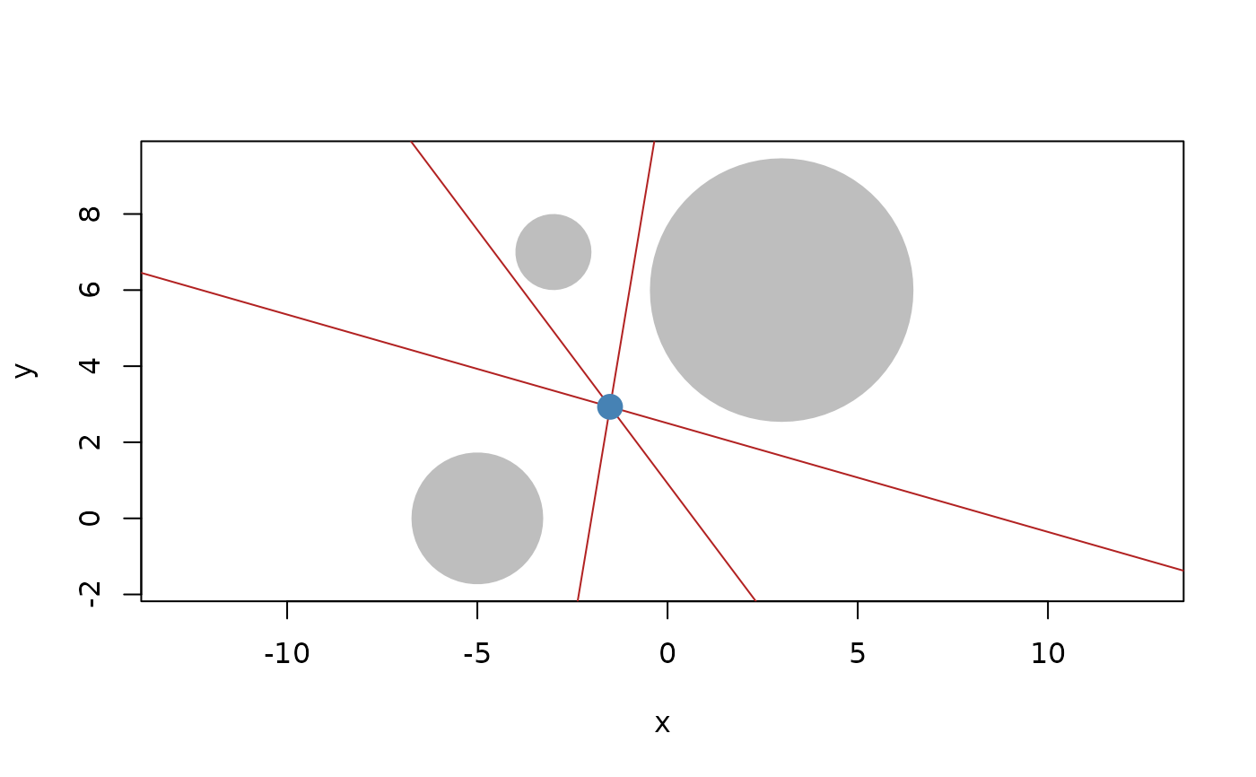
# Example visualisation of radical points and lines
c1 <- circle(point(3, 6), 12)
c2 <- circle(point(-5, 0), 3)
c3 <- circle(point(-3, 7), 1)

plot(c(c1, c2, c3), bg = "grey", fg = NA)
euclid_plot(c(
  radical(c1, c2),
  radical(c2, c3),
  radical(c1, c3)
), col = "firebrick")
euclid_plot(radical(c1, c2, c3), pch = 16, cex = 2, col = "steelblue")