Euclid is a package for computational geometry in R. Not just that, it is also the foundation for a whole universe of packages devoted to specific subsets of computational geometry. In order to understand this universe, you must at least have a passing understanding of euclid. Fear not, the purpose of the euclid API is to make computational geometry as R-like as possible so it seems like triangles, segments, lines, etc. are just vectors in line with other basic R vectors like logicals and numerics.
The foundation
At the heart of euclid is a range of new atomic vector types that
describe geometric primitives. These primitives are e.g. segments,
points, triangles, planes, circles, etc. Some of these exists in
variants for both 2D and 3D space, while others are confined to either
of these (e.g. a plane is only defined in 3D space). The geometries can
be created through their constructors or by coercing one geometry to
another. To create a point, you can supply its x and
y coordinates:
library(euclid)
p <- point(c(5, 3, 7), 2)
p
#> <2D points [3]>
#> [1] <x:5, y:2> <x:3, y:2> <x:7, y:2>
As you can see, the input arguments are recycled, so that all 3
points here have the same y coordinate. Note that the input
arguments are not named and only rely on their positions. This might
seem odd in the case of points where using x and
y as argument names are obvious, but it becomes clear soon
why this approach doesn’t scale.
A vector can, as with points, be created from a set of x
and y coordinates, but you could also create it from a
vector of points:
v <- vec(p)
v
#> <2D vectors [3]>
#> [1] <x:5, y:2> <x:3, y:2> <x:7, y:2>
As the complexity of the geometry increases so does its number of ways to construct it. A circle in 2D can for instance be constructed from a point and a radius, but it can just as well be constructed from three points in which case it will created the unique circle that goes through all three points (unless they are co-linear):
# Create 3 new points because the ones defined above are co-linear
p <- point(
  c(3, 6, 2),
  c(7, 1, 5)
)
circ <- circle(p[1], p[2], p[3])
circ
#> <2D circles [1]>
#> [1] <x:5.5, y:4.5, r2:12.5>

plot(circ)
plot(p, add = TRUE)
It is advised to consult the documentation for each geometry to see the different ways in which they can be created.
Extracting values
While the geometries in euclid are atomic, they still encode
information that can be extracted. For instance, you might be interested
in getting the y coordinates of the points in a vector.
Such information can be accessed with def(), short for
definition:
def(p, 'y')
#> <exact numerics [3]>
#> [1] 7 1 5
The definition names of each geometry can be accessed with
definition_names():
definition_names(circ)
#> [1] "x"  "y"  "r2"
You can also use def() to alter the geometries:
def(circ, "r2") <- 1
circ
#> <2D circles [1]>
#> [1] <x:5.5, y:4.5, r2:1>
Another type of information that can be extracted are the points that
make up the geometry. For circles, that would be the center, for
segments it would be either the start or end, etc. This can be accessed
with the vert() function:
vert(circ)
#> <2D points [1]>
#> [1] <x:5.5, y:4.5>
For most geometries there is only one vertex to access, but some have
several (e.g. segments). The number of vertices in a geometry can be
found out with the cardinality() function:
tri <- triangle(p[1], p[2], p[3])
cardinality(tri)
#> [1] 3
vert(tri, 3)
#> <2D points [1]>
#> [1] <x:2, y:5>
If you do not specify a vertex index it will extract all the vertices at once:
vert(tri)
#> <2D points [3]>
#> [1] <x:3, y:7> <x:6, y:1> <x:2, y:5>
Like def(), vert() can also be used for
altering the geometries:
For geometries consisting of multiple vertices (segments, triangles, tetrahedrons, iso rectangles, and iso cuboids) it is also possible to extract the edges of the geometries as a segments vector:
edge(tri, 1)
#> <2D segments [1]>
#> [1] [<x:0, y:0>, <x:6, y:1>]
Again, not specifying an index extracts them all:
edge(tri)
#> <2D segments [3]>
#> [1] [<x:0, y:0>, <x:6, y:1>] [<x:6, y:1>, <x:2, y:5>] [<x:2, y:5>, <x:0, y:0>]
edge() cannot be used to alter geometries - for that
you’d need to alter each vertex individually.
A last choice is to convert the geometry to a matrix. This will put all the definitions in a separate column and create as many rows as the cardinality of the geometry for each element in the vector:
as.matrix(tri)
#>      [,1] [,2]
#> [1,]    0    0
#> [2,]    6    1
#> [3,]    2    5
One thing to note with this last approach is that the output will be
given in standard R numerics, whereas def() will output
something else… read on!
A note on exactness
You might have paused at the output of def():
def(tri, 'x')
#> <exact numerics [3]>
#> [1] 0 6 2
This doesn’t look like a standard R vector. It isn’t! The output is an exact numeric, which is a new type of numeric vector introduced with euclid. The reason for the inclusion of this is that floating points can cause all types of issues with compounding imprecision. Normally this is not an issue in programming (until it is), but in computational geometry it is an absolute nightmare to deal with. Imagine creating a plane based on three points in 3D space, only to find that one of the points doesn’t lie on that plane… not fun!
# Floating point issues at play
a <- c(12, 10, 2) / 10
a[1] - a[2] == a[3]
#> [1] FALSE

# None of that in euclid
b <- exact_numeric(c(12, 10, 2)) / 10
b[1] - b[2] == b[3]
#> [1] TRUE
As you can see, you can perform arithmetic on exact numerics in the
way you are used to, and great care has been put in making them behave
just like numeric vectors. There are limits, however, since some math
operations cannot be performed while ensuring exactness,
e.g. sqrt() (This is also why the radius of circles are
given as the squared radius). If this is needed it is necessary to
convert to standard numerics, but be aware that any exactness has been
lost at that point.
Everything in euclid is based on exact numbers and thus doesn’t
exhibit any issues related to floating point numbers, as long as you
don’t convert back and forth between euclid and R types. In the case
exact results are not possible, euclid will sometimes provide a function
prefixed with approx_* that returns standard numerics
(e.g. approx_area()). Approx in this sense shouldn’t mean
that it is only calculating an approximation, but simply that the answer
cannot be given exact, i.e. the result of approx_area() is
true down to the precision of the numeric type (2.220446^{-16}).
Working with geometries
While having geometries as atomic vectors is in itself a nice thing, it is what we can do with them that are truly interesting. As said in the introduction the intent is that specialized algorithms are relegated to their own packages. However, euclid comes with a slew of basic algorithms that can get you pretty far.
Predicates
Predicates are at the heart of many geometric algorithms: Do these two geometries intersect?, Does this point lie to the right of this line? Are this line parallel with this plane? euclid implement many of these, both as standard functions and infix operators:
is_degenerate()queries if the geometry is validhas_on()/%is_on%queries if one geometry lies on the boundary of anotherhas_inside()/%is_inside%queries if one geometry lies inside anotherhas_outside()/%is_outside%queries if one geometry lies outside anotherhas_on_positive_side()/%is_on_positive_side%queries if one geometry lies on the positive side of anotherhas_on_negative_side()/%is_on_negative_side%like above but for the negative sideis_constant_in()queries whether a geometry doesn’t vary along an axisparallel()queries if two geometries are parallelcollinear()/coplanar()queries if geometries are collinear or coplanarturns_left()/turns_right()queries if a progression of points turns right or lefthas_intersection()/%is_intersecting%queries if two geometries are intersecting
We will not showcase all of these - the documentations all have examples. But just to show how they are used we can see how point inclusion in a triangle can be queried:
p <- point(sample(10, 50, TRUE), sample(10, 50, TRUE))
t <- triangle(point(1, 5), point(10, 10), point(5, 1))
plot(t, col = "grey", border = NA)
euclid_plot(p[p %is_on% t], pch = 16, col = "firebrick")
euclid_plot(p[p %is_inside% t], pch = 16, col = "steelblue")
euclid_plot(p[p %is_outside% t], pch = 16, col = "goldenrod")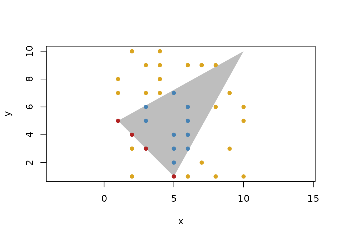
Locations
One or a set of geometries can give rise to a new geometry, e.g. a triangle has a centroid, two points gives rise to a bisector, etc. euclid has a set of location functions that returns new geometries based on the input:
circumcenter()can calculate the circumcenter of triangles, tetrahedrons, or point setsbarycenter()calculates the center of mass off a set of weighted pointsbisector()splits the space in two based on two pointscentroid()calculates the geometric mean of points, a triangle, or a tetrahedronequidistant_line()calculates the line that remains at equal distance to 2 or 3 points along its trajectoryradical()calculates the radical line or plane of two circles/spheres or the radical point of three circles/spheres
c1 <- circle(point(3, 6), 12)
c2 <- circle(point(-5, 0), 3)
c3 <- circle(point(-3, 7), 1)

plot(c(c1, c2, c3), bg = "grey", fg = NA)
plot(c(radical(c1, c2), radical(c2, c3), radical(c1, c3)), col = "firebrick", add = TRUE)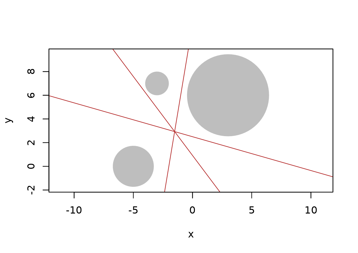
Intersections
Whether or not two geometries intersect, and how, is often needed. We
saw in the predicates section that euclid has
functionality for calculation if two geometries intersect. It
can, however, also return the actual intersection. In general, the
return value of an intersection calculation can be quite heterogeneous,
as e.g. two segments can intersect in either a point (if the cross), a
new segment (if they are parallel and overlap), or not at all. Because
of this intersection() returns a list of geometries instead
of a geometry vector. If type stability is of concern, there are
versions for that (e.g. intersection_point()), but with
these it is not possible to distinguish between lack of intersection and
an intersection of the wrong type (both are converted to
NA).
t <- triangle(point(0, 0), point(1, 1), point(0, 1))
l <- line(1, -1, c(0, 1, 2))
intersection(t, l)
#> [[1]]
#> <2D segments [1]>
#> [1] [<x:1, y:1>, <x:0, y:0>]
#>
#> [[2]]
#> <2D points [1]>
#> [1] <x:0, y:1>
#>
#> [[3]]
#> NULL

intersection_segment(t, l)
#> <2D segments [3]>
#> [1] [<x:1, y:1>, <x:0, y:0>] <NA>                     <NA>
Projections
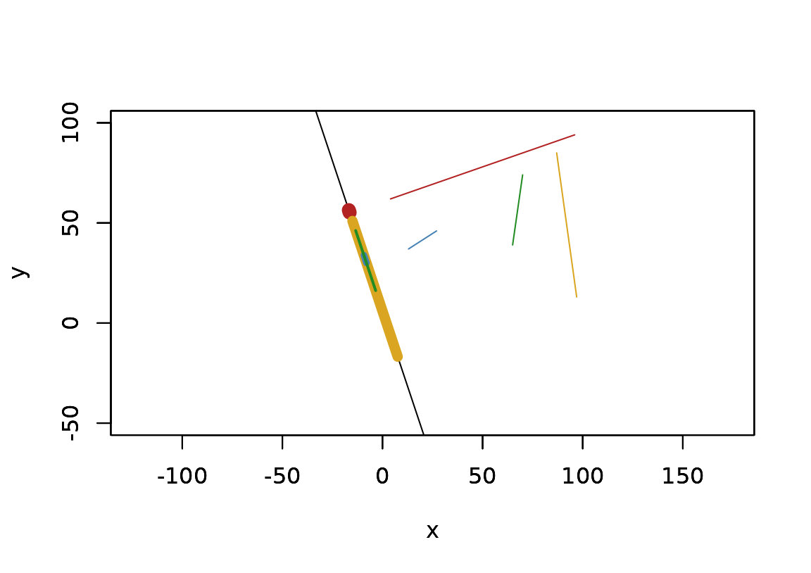
Geometries may be projected to lines are planes, which means their coordinates are moved to their closest location on a line or plane. There is also a variant where 3D geometries are converted to their 2D counterpart by mapping their location to a plane.
p <- point(sample(100, 8), sample(100, 8))
s <- segment(p[1:4], p[5:8])
l <- line(3, 1, -6)

s_proj <- project(s, l)
s_proj
#> <2D segments [4]>
#> [1] [<x:-16.8, y:56.4>, <x:-16.4, y:55.2>]
#> [2] [<x:-15, y:51>, <x:7.6, y:-16.8>]
#> [3] [<x:-9.3, y:33.9>, <x:-8, y:30>]
#> [4] [<x:-3.4, y:16.2>, <x:-13.4, y:46.2>]

plot(l, xlim = c(-50, 100), ylim = c(-50, 100))
plot(s, col = c("firebrick", "goldenrod", "steelblue", "forestgreen"), add = TRUE)
plot(
  s_proj,
  col = c("firebrick", "goldenrod", "steelblue", "forestgreen"),
  lwd = seq(10, 2, length.out = 4),
  add = TRUE
)
Transformations
Geometries exists in euclidean space (at least those provided by euclid does), and as such can be moved around. Euclid supports all types of affine transformations, with the caveats that circles and spheres remain as circles and spheres even when stretched or sheared (i.e. those transformations only affect their location).
Euclid has support for creating and combining affine transformation
matrices through the affine transformation matrix vector type, which
thus allows vectorised transformations of your geometries using the
transform() generic.
tri <- triangle(point(1, 0), point(3, 1), point(2, 3))

scale <- affine_scale(2)

tri_scaled <- transform(tri, scale)

plot(c(tri, tri_scaled), lty = c(2, 1))
center <- centroid(tri)

move_to_middle <- affine_translate(-vec(center))
# Transformations can be stacked by multiplication in reverse order
scale_center <- inverse(move_to_middle) * scale * move_to_middle

tri_scaled2 <- transform(tri, scale_center)

plot(c(tri, tri_scaled2), lty = c(2, 1))
All the rest
There are more things we haven’t discussed, as some of it are specific to certain geometries, such as querying whether a direction lies between two other directions, or adding vectors together, or sorting point, or interpolating between geometries, or getting bounding boxes, or… you get the idea. Please consult the thorough documentation to dive deeper into the possibilities of euclid