Query location of points relative to geometry
Source:R/geometry_predicates.R
location_predicates.RdPoint predicates is at the heart of many geometry algorithms. These set of functions allows you to query the location of points relative to a given geometry vector. The functions are provided as both regular and binary operators.
Usage
has_on(x, y)

y %is_on% x

has_inside(x, y)

y %is_inside% x

has_outside(x, y)

y %is_outside% x

has_on_positive_side(x, y)

y %is_on_positive_side% x

has_on_negative_side(x, y)

y %is_on_negative_side% xDetails
There are two types of location predicates:
Containment (inside and outside)
Queries whether a point is inside or outside the boundary defined by the geometry. In 2D it is defined for geometries that have an area, In 3D it is defined for geometries that has a volume. This means that containment is defined for 2D circles but not 3D circles.
Orientation (positive and negative)
Queries whether a point lies on the positive or negative side of a geometry. It is defined for geometries that splits the dimensional space in two. This means that it is not defined for rays, segments, etc with a finite length.
For both types of predicates there are also the condition that the point lies on the geometry. This predicate is equivalent for both types of predicates and is defined for all geometries that has a location. This means that e.g. directions and vectors do not define this predicate.
See also
Other Predicates:
collinear(),
constant_in,
geometry_class,
geometry_turns,
has_intersection(),
in_order(),
is_degenerate(),
parallel()
Examples
p <- point(sample(10, 50, TRUE), sample(10, 50, TRUE))
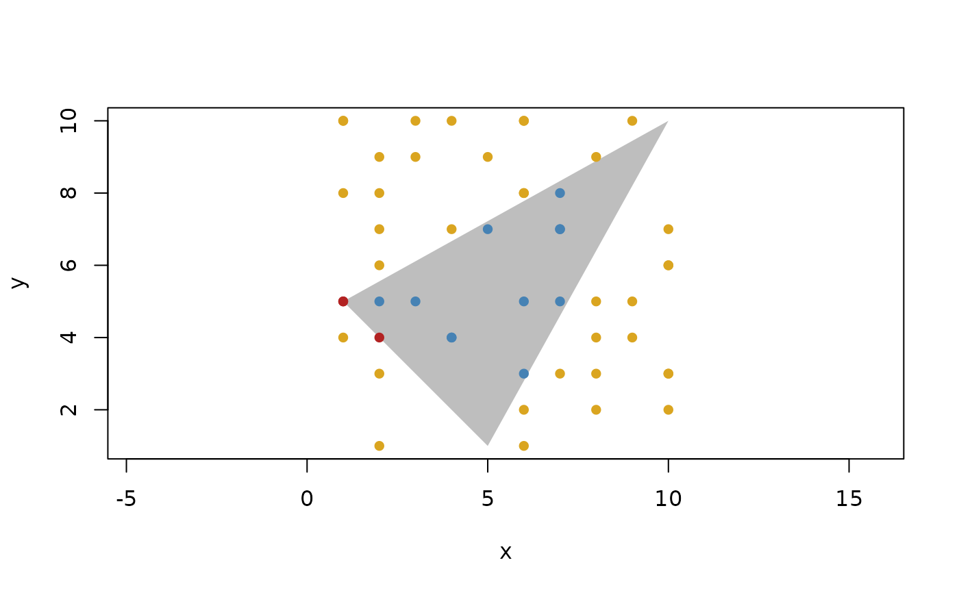
t <- triangle(point(1, 5), point(10, 10), point(5, 1))

plot(t, col = "grey", border = NA)
euclid_plot(p[p %is_on% t], pch = 16, col = "firebrick")
euclid_plot(p[p %is_inside% t], pch = 16, col = "steelblue")
euclid_plot(p[p %is_outside% t], pch = 16, col = "goldenrod")


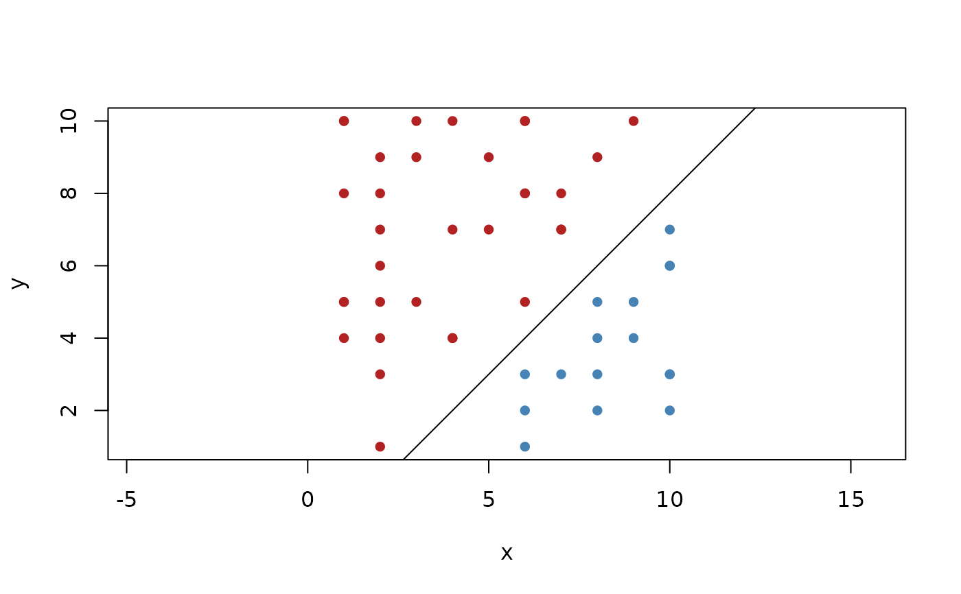
l <- line(-1, 1, 2)
plot(l, xlim = c(1, 10), ylim = c(1, 10))
euclid_plot(p[p %is_on_positive_side% l], pch = 16, col = "firebrick")
euclid_plot(p[p %is_on_negative_side% l], pch = 16, col = "steelblue")
